03 Hartree-Fock Closed-Shell SCF Procedure
The purpose of this project is to provide a deeper understanding of (restricted) Hartree-Fock theory by demonstrating a simple implementation of the self-consistent-field (SCF) method. The theoretical background can be found in Ch. 3 of the text by Szabo and Ostlund or in the nice set of on-line notes written by David Sherrill. A concise set of instructions for this project may be found here.
Original authors (Crawford, et al.) thank Dr. Yukio Yamaguchi of the University of Georgia for the original version of this project.
This project could be a challenging one. Although it is somehow easy to achieve each steps, the number of steps is quite large. You may well possibly have done all tasks, but confuse on how and why iterative SCF could be written in this way. You are encouraged to review this project once you’ve done all steps.
The test case used in the following discussion is for a water molecule with a bond-length of \(1.1 {\buildrel_{\circ} \over{\mathsf{A}}}\) and a bond angle of \(104.0 {}^\circ\) with an STO-3G basis set. The input to the project consists of the nuclear repulsion energy (input/h2o/STO-3G/enuc.dat) and pre-computed sets of one- and two-electron integrals: overlap integrals (input/h2o/STO-3G/s.dat), kinetic-energy integrals (input/h2o/STO-3G/t.dat), nuclear-attraction integrals (input/h2o/STO-3G/v.dat), electron-electron repulsion integrals (input/h2o/STO-3G/eri.dat).
Multiple ways to achieve a task
From this project, it could be multiple ways to achieve a task. What multiple means here is that one could
either read integrals from input file, or from PySCF’s integral interface;
either do (high-dimension) tensor contraction by extremely powerful
numpy.einsum(NumPy API), or by simply for-looping, or hybrid for-looping and 2-dimension matrix manipulation;format outputs by his own style (with most important values unchanged to the reference solution output);
etc.
Multiple approaches could arrive to the almost same solution, and every approach is appreciated. The reader may develop his/hers own coding style. However, as author of the documentation, there’s still some partiality for using PySCF’s integral interface and using numpy.einsum.
In this project, using module pyscf.scf is prohibited. Using pyscf.gto is permitted. The structure of this project is slightly changed compared to the original project 03.
# Following os.chdir code is only for thebe (live code), since only in thebe default directory is /home/jovyan
import os
if os.getcwd().split("/")[-1] != "Project_03":
    os.chdir("source/Project_03")
from solution_03 import Molecule as SolMol
# Following code is called for numpy array pretty printing
from pyscf import gto
import numpy as np
from scipy.linalg import fractional_matrix_power
from pprint import pp  # Data Pretty Printer, as it says
from typing import Dict, Tuple  # only used in type infer
np.set_printoptions(precision=7, linewidth=120, suppress=True)
sol_mole = SolMol()
sol_mole.construct_from_dat_file("input/h2o/STO-3G/geom.dat")
sol_mole.path_dict = {
    "enuc": "input/h2o/STO-3G/enuc.dat",
    "s": "input/h2o/STO-3G/s.dat",
    "t": "input/h2o/STO-3G/t.dat",
    "v": "input/h2o/STO-3G/v.dat",
    "eri": "input/h2o/STO-3G/eri.dat",
    "mux": "input/h2o/STO-3G/mux.dat",
    "muy": "input/h2o/STO-3G/muy.dat",
    "muz": "input/h2o/STO-3G/muz.dat",
}
Notation Convention
It is important to make notation convention clear at the very beginning, or otherwise one may could have taken the wrong comprehension all the time reading article or documentation even without recognizing that. Here we make some essential, but not all, notations that we use in the documents thereafter. Meaning of some notations to some readers maybe not clear or familiar. These notations would be discussed in later sections or documents.
\(\mu, \nu, \kappa, \lambda\): Atomic orbitals. These notations are different to Szabo and Ostlund’s \(\mu, \nu, \sigma, \lambda\). Decision of changing \(\sigma\) to \(\kappa\) based on the convention that \(\sigma\) is more abused to be notation of orbital spin.
\(i, j, k, l, ...\): Occupied orbitals. These notations are more accepted nowadays, which are different to Szabo and Ostlund’s \(a, b, c, ...\).
\(a, b, c, d, ...\): Virtual orbitals (un-occupied orbitals). The same reason to above.
\(p, q, r, s, m\): All accepted orbitals.
\(n_\mathrm{occ}, n_\mathrm{vir}, n_\mathrm{AO}, n_\mathrm{MO}\): Number of occupied, virtual, atomic and molecular orbitals, respectively.
\(A, B, C, M\): Atom subscripts. These notations are different to the previous projects’ \(i, j, k, ...\)
\(\boldsymbol{r}, \boldsymbol{R}_A\): Coordinate of electron and nucleus of atom \(A\), respectively.
\(Z_A\): Atomic charge of atom \(A\).
In the documentation, we will not learn frozen orbitals. So division of occupied and virtual is sufficient.
Molecule Object Initialization
In this project, we may use the updated Molecule initialization. Since these are technical details, we toggle the code and explanation below.
class Molecule:

    def __init__(self):
        self.atom_charges = NotImplemented  # type: np.ndarray
        self.atom_coords = NotImplemented   # type: np.ndarray
        self.natm = NotImplemented          # type: int
        self.mol = NotImplemented           # type: gto.Mole
        self.path_dict = NotImplemented     # type: Dict[str, str]
        self.nao = NotImplemented           # type: int
        self.charge = 0                     # type: int
        self.nocc = NotImplemented          # type: int

    def construct_from_dat_file(self, file_path: str):
        # Same to Project 01
        with open(file_path, "r") as f:
            dat = np.array([line.split() for line in f.readlines()][1:])
            self.atom_charges = np.array(dat[:, 0], dtype=float).astype(int)
            self.atom_coords = np.array(dat[:, 1:4], dtype=float)
            self.natm = self.atom_charges.shape[0]


mole = Molecule()
mole.construct_from_dat_file("input/h2o/STO-3G/geom.dat")
The meaning of attributes of Molecule are:
atom_charges: Array to store atomic chargesatom_coords: Matrix to store coordinates of atomsnatm: Number of atomsmol:pyscf.gto.Moleinstance, which describes molecular and basis information; only used in PySCF approachespath_dict: Dictionary of file path which containing integral, energy, …; only used in reading-input approachesnao: Number of atomic orbitals \(n_\mathrm{AO}\)charge: Molecular charge (\(\mathsf{NH_4^+}\) contains +1 charge and \(\mathsf{NO_3^-}\) contains -1 charge); in most cases we just use neutral moleculesnocc: Number of occupied orbitals \(n_\mathrm{occ}\)
Readers may be familier with the first three attributes which we have extensively used in Project 01 and Project 02. One may call Molecule.construct_from_dat_file to initialize these three attributes. For demonstration, we use STO-3G water molecule which is instantiated as variable mole.
Extra initialization: PySCF approach
In PySCF, molecule and basis information is stored in pyscf.gto.Mole (PySCF API) instance. For example, the water molecule and basis STO-3G (the same to de demonstrated molecule) could be instantiated by
mol = gto.Mole()
mol.unit = "Bohr"
mol.atom = """
8   0.000000000000  -0.143225816552   0.000000000000
1   1.638036840407   1.136548822547  -0.000000000000
1  -1.638036840407   1.136548822547  -0.000000000000
"""
mol.basis = "STO-3G"
mol.build()
Though the molecule can be manually instantiated, we still need a method function in Molecule, using existing mole.atom_charges and mole.atom_coords and external basis "STO-3G", to build the pyscf.gto.Mole instance and store in mole.mol attribute.
Note that we just discuss closed-shell situation, so we set mol.spin = 0. The convention of molecular spin in different softwares might be quite deviated. In PySCF, mol.spin means number of alpha electrons minus beta electrons.
Class pyscf.gto.Mole can be extremely useful and convenient for this documentation, as almost all electron integrals can be called by method function pyscf.gto.Mole.intor in only one short line of code.
Implementation
Reader should fill all NotImplementedError in the following code:
def obtain_mol_instance(mole: Molecule, basis: str, verbose=0):
    # Input: Basis string information
    #        (for advanced users, see PySCF API, this could be dictionary instead of string)
    # Attribute modification: Obtain `pyscf.gto.Mole` instance `mole.mol`
    mol = gto.Mole()
    mol.unit = "Bohr"
    raise NotImplementedError("About 2~20 lines of code, where `mol.atom` and `mol.basis` need to be defined")
    mol.charge = mole.charge
    mol.spin = 0
    mol.verbose = verbose
    mole.mol = mol.build()

Molecule.obtain_mol_instance = obtain_mol_instance
Solution
sol_mole.obtain_mol_instance(basis="STO-3G")
print("=== Coordinate ===")
print(sol_mole.mol.atom_coords())
print("=== Atomic Charges ===")
print(sol_mole.mol.atom_charges())
print("=== Basis Detail ===")
pp(sol_mole.mol._basis)
=== Coordinate ===
[[ 0.        -0.1432258  0.       ]
 [ 1.6380368  1.1365488  0.       ]
 [-1.6380368  1.1365488  0.       ]]
=== Atomic Charges ===
[8 1 1]
=== Basis Detail ===
{'H': [[0,
        [3.42525091, 0.15432897],
        [0.62391373, 0.53532814],
        [0.1688554, 0.44463454]]],
 'O': [[0,
        [130.70932, 0.15432897],
        [23.808861, 0.53532814],
        [6.4436083, 0.44463454]],
       [0,
        [5.0331513, -0.09996723],
        [1.1695961, 0.39951283],
        [0.380389, 0.70011547]],
       [1,
        [5.0331513, 0.15591627],
        [1.1695961, 0.60768372],
        [0.380389, 0.39195739]]]}
Extra initialization: Read-input approach
Molecule.charge and Molecule.path_dict should be expicitly defined by caller. If you decided to use PySCF generating integrals, and not using pre-generated integrals in directory input/h2o/STO-3G, you are prefered to set this value to None or NotImplemented. Otherwise, you may explicitly state paths manually as the following toggled code:
mole.path_dict = {
    "enuc": "input/h2o/STO-3G/enuc.dat",
    "s": "input/h2o/STO-3G/s.dat",
    "t": "input/h2o/STO-3G/t.dat",
    "v": "input/h2o/STO-3G/v.dat",
    "eri": "input/h2o/STO-3G/eri.dat",
    "mux": "input/h2o/STO-3G/mux.dat",
    "muy": "input/h2o/STO-3G/muy.dat",
    "muz": "input/h2o/STO-3G/muz.dat",
}
Step 1: Nuclear Repulsion Energy
Nuclear Repulsion Energy can be determined as (Szabo, eq 3.185)
PySCF approach
PySCF provides a method function that directly calculate nuclear repulsion energy pyscf.gto.Mole.energy_nuc.
Read-Input approach
File input/h2o/STO-3G/enuc.dat contains nuclear repulsion energy.
Direct approach
Actually programming nuclear repulsion energy is not a difficult job. One can simply write two for loops to achieve the task. However, there could be a bonus challenge, only using matrix/tensor operation without for loop, to calculate the energy. The point is
where we (unphysically) define \(R_{AB} = +\infty\) if \(A = B\).
Implementation
Reader should fill all NotImplementedError in the following code:
def eng_nuclear_repulsion(mole: Molecule) -> float:
    # Output: Nuclear Repulsion Energy
    # PySCF       Exactly 1 line of code
    # Read-Input  Exactly 2 or 3 lines of code
    # Direct      About 2~10 lines of code
    raise NotImplementedError("Various approaches may have different lines of code")

Molecule.eng_nuclear_repulsion = eng_nuclear_repulsion
Solution
sol_mole.eng_nuclear_repulsion()
8.00236706181077
Step 2: One-Electron Integrals
Read various atomic orbital (AO) electron integrals.
Overlap s
Kinetic Integral t
Nuclear-Attraction Integral v
Then form the core Hamiltonian:
Hint 1: Proper dimension of matrices
It could be important to know how large the matrix is, before we handle electron integrals.
To get the dimension of matrix from fomular, for example overlap \(S_{\mu \nu}\), we should take a look at subscripts \(\mu \nu\), where it indicates dimension is related to \((\mu, \nu)\). Since \(\mu, \nu\) are atomic orbitals, dimension of overlap should be \((n_\mathrm{AO}, n_\mathrm{AO})\).
However, \(n_\mathrm{AO}\) can not be apparently got (since it requires summation of basis; however not everyone is required to recite how many basis functions are for Oxygen or Hydrogen DZP, or whether Uraine could be described by STO-3G).
For PySCF approach, one can use pyscf.gto.Mole.nao attribute to obtain \(n_\mathrm{AO}\). For read-input approach, one could read the last line of file, for example in input/h2o/STO-3G/t.dat:
7 7 0.760031883566609
Then we should know there are 7 atomic orbitals, i.e. \(n_\mathrm{AO} = 7\).
One may implement a short method function obtain_nao to store number of atomic orbitals.
Hint 2: General function to store 1-electron integral
Here we need to read three integrals. Since these three integrals are stored in exactly the same way, so we can make some kind of abstraction, i.e. a function which could not only read overlap, but also read kinetic or nuclear attraction integrals.
Recall that all these 1-electron integrals are symmetric matrices (or permutationally unique), so in .dat files, only lower-triangle part is stored. However, we prefer to store full matrices in computer memory for coding convenience. Also note that the AO indices on the integrals in the files start with 1 rather than 0.
One may implement a function read_integral_1e to read 1-electron integrals.
Hint 3: PySCF function pyscf.gto.Mole.intor
In PySCF, integrals can be generated by elegent function pyscf.gto.Mole.intor. For example, overlap integral can be generated in following code.
>>> sol_mole.mol.intor("int1e_ovlp")
array([[ 1.       ,  0.2367039,  0.       , -0.       ,  0.       ,  0.0384056,  0.0384056],
       [ 0.2367039,  1.       ,  0.       ,  0.       ,  0.       ,  0.3861388,  0.3861388],
       [ 0.       ,  0.       ,  1.       ,  0.       ,  0.       ,  0.2684382, -0.2684382],
       [-0.       ,  0.       ,  0.       ,  1.       ,  0.       ,  0.2097269,  0.2097269],
       [ 0.       ,  0.       ,  0.       ,  0.       ,  1.       ,  0.       ,  0.       ],
       [ 0.0384056,  0.3861388,  0.2684382,  0.2097269,  0.       ,  1.       ,  0.1817599],
       [ 0.0384056,  0.3861388, -0.2684382,  0.2097269,  0.       ,  0.1817599,  1.       ]])
Full list of supported integrals are listd in PySCF API. What we need in this step is
int1e_ovlp: overlapint1e_kin: kinetic integralint1e_nuc: nuclear-attraction integral
Implementation
You may either want to store the integrals by Molecule attributes (in computer memory), or generate integrals on-the-fly (i.e. generate integrals when we aquire them, otherwise they are not stored in computer memory). The inplementation of reference solution uses the latter way.
Reader should fill all NotImplementedError in the following code:
def obtain_nao(mole: Molecule, file_path: str=NotImplemented):
    # Input: Any integral file (only used in read-input approach, pyscf approach could simply leave NotImplemented)
    # Attribute Modification: `nao` number of atomic orbitals
    raise NotImplementedError("About 1~3 lines of code")

Molecule.obtain_nao = obtain_nao
def read_integral_1e(mole: Molecule, file_path: str) -> np.ndarray:
    # Input: Integral file
    # Output: Symmetric integral matrix
    raise NotImplementedError("About 6~15 lines of code; PySCF approach does not need to implement this function")

Molecule.read_integral_1e = read_integral_1e
Reader should choose one approach and remove NotImplementedError in the following code:
def integral_ovlp(mole: Molecule) -> np.ndarray:
    # Output: Overlap
    # PySCF        return mole.mol.intor("int1e_ovlp")
    # Read-Input   return mole.read_integral_1e(mole.path_dict["s"])
    raise NotImplementedError("Choose one approach")

def integral_kin(mole: Molecule) -> np.ndarray:
    # Output: Kinetic Integral
    # PySCF        return mole.mol.intor("int1e_kin")
    # Read-Input   return mole.read_integral_1e(mole.path_dict["t"])
    raise NotImplementedError("Choose one approach")

def integral_nuc(mole: Molecule) -> np.ndarray:
    # Output: Nuclear Attraction Integral
    # PySCF        return mole.mol.intor("int1e_nuc")
    # Read-Input   return mole.read_integral_1e(mole.path_dict["v"])
    raise NotImplementedError("Choose one approach")

def get_hcore(mole: Molecule) -> np.ndarray:
    # Output: Hamiltonian Core
    return mole.integral_kin() + mole.integral_nuc()

Molecule.integral_ovlp = integral_ovlp
Molecule.integral_kin = integral_kin
Molecule.integral_nuc = integral_nuc
Molecule.get_hcore = get_hcore
Solution
sol_mole.obtain_nao()
sol_mole.nao
7
sol_mole.get_hcore()
array([[-32.5773954,  -7.5788328,  -0.       ,  -0.0144738,   0.       ,  -1.2401023,  -1.2401023],
       [ -7.5788328,  -9.2009433,  -0.       ,  -0.1768902,   0.       ,  -2.9067098,  -2.9067098],
       [  0.       ,   0.       ,  -7.4588193,   0.       ,   0.       ,  -1.6751501,   1.6751501],
       [ -0.0144738,  -0.1768902,   0.       ,  -7.4153118,   0.       ,  -1.3568683,  -1.3568683],
       [  0.       ,   0.       ,   0.       ,   0.       ,  -7.3471449,   0.       ,   0.       ],
       [ -1.2401023,  -2.9067098,  -1.6751501,  -1.3568683,   0.       ,  -4.5401711,  -1.0711459],
       [ -1.2401023,  -2.9067098,   1.6751501,  -1.3568683,   0.       ,  -1.0711459,  -4.5401711]])
Step 3: Two-Electron Integrals
Read the two-electron repulsion integrals (electron repulsion integral, ERI) from the input/h2o/STO-3G/eri.dat file. The integrals in this file are provided in Mulliken notation over real AO basis functions:
Hence, the integrals obey the eight-fold permutational symmetry relationships:
and only the permutationally unique integrals are provided in the file, with the restriction that, for each integral, the following relationships hold:
where
Although two-electron integrals may be stored efficiently in a one-dimensional array and the above relationship, we still use full dimension (i.e. dimension \((\mu, \nu, \kappa, \lambda)\) or \((n_\mathrm{AO}, n_\mathrm{AO}, n_\mathrm{AO}, n_\mathrm{AO})\)) to store the two-electron integral tensor, for coding convenience.
If you prefer smaller memory buffer but somehow greater cost of computational efficiency cost and code complexity, original project 03 provides some insights on this.
Implementation
Reader should fill all NotImplementedError in the following code:
def read_integral_2e(mole: Molecule, file_path: str) -> np.ndarray:
    # Input: Integral file
    # Output: 8-fold symmetric 2-e integral tensor
    raise NotImplementedError("About 6~20 lines of code; PySCF approach does not need to implement this function")

Molecule.read_integral_2e = read_integral_2e
Reader should choose one approach and remove NotImplementedError in the following code:
def integral_eri(mole: Molecule) -> np.ndarray:
    # Output: Electron repulsion integral
    # PySCF        return mole.mol.intor("int2e")
    # Read-Input   return mole.read_integral_2e(mole.path_dict["eri"])
    raise NotImplementedError("Choose one approach")

Molecule.integral_eri = integral_eri
Solution
Here we only print one sub-matrix in the electron repulsion integral:
sol_mole.integral_eri()[0, 3]
array([[-0.       , -0.       ,  0.       ,  0.0244774,  0.       ,  0.0006308,  0.0006308],
       [-0.       , -0.       ,  0.       ,  0.0378086,  0.       ,  0.0033729,  0.0033729],
       [ 0.       ,  0.       , -0.       ,  0.       ,  0.       ,  0.0017449, -0.0017449],
       [ 0.0244774,  0.0378086,  0.       , -0.       ,  0.       ,  0.0087746,  0.0087746],
       [ 0.       ,  0.       ,  0.       ,  0.       , -0.       ,  0.       ,  0.       ],
       [ 0.0006308,  0.0033729,  0.0017449,  0.0087746,  0.       ,  0.0063405,  0.0017805],
       [ 0.0006308,  0.0033729, -0.0017449,  0.0087746,  0.       ,  0.0017805,  0.0063405]])
Step 4: Build the Orthogonalization Matrix
Diagonalize the overlap matrix:
where \(\mathbf{L}\) is the matrix of eigenvectors (columns) and \(\mathbf{\Lambda}\) is the diagonal matrix of corresponding eigenvalues.
Build the symmetric orthogonalization matrix using (Szabo and Ostlund, eq 3.167):
where dagger \(\dagger\) denotes the matrix transpose.
Scipy approach
Actually this process is exactly the same to matrix power (with fractional exponent). This could be done simply by scipy.linalg.fractional_matrix_power (SciPy API)
For proper definition of matrix power, see Matrix function: Diagonalizable matrices. Another useful definition could be Cauchy integral from complex analysis; actually this definition is applied to -1/2 power of matrix in direct random phase approximation (dRPA) correlation energy calculation. Well, in this project, diagonalizable matrix scheme should be sufficient.
Direct approach
For diagonal matrix, -1/2 power of matrix is equal to -1/2 power to its diagonal values. For example,
So, not all matrices could be implied with -1/2 power. Only those matrices which eigenvalues are non-zero could be implied with -1/2 power. If negative eigenvalues exists, the matrix implied with -1/2 power could be complex.
Note on orthogonalization matrix
Our cases in this project is somehow well-behaved. So, the overlap matrices \(\mathbf{S}\) would have positive eigenvalues, and orthogonalization matrix is simply symmetric with dimension \((n_\mathrm{AO}, n_\mathrm{AO})\). Thus number of molecular orbital \(n_\mathrm{MO}\) is equal to \(n_\mathrm{AO}\).
However, when basis become larger, overlap matrices \(\mathbf{S}\) could be ill-behaved (linear dependent, or some eigenvalues very close to zero), thus \(\mathbf{S}^{-1/2}\) can be numerical instable. Solution to this behavior is discussed in Szabo and Ostlund roughly, around eq 3.172. In this situation, \(n_\mathrm{MO} < n_\mathrm{AO}\).
It is important to know that, though in this documentation, \(n_\mathrm{MO} = n_\mathrm{AO}\) in most situations, they are essentially two different concepts and does not need to be equal to each other. Molecular orbitals is linear combinition of atomic orbitals (LCAO). Computationally or say in practice, these two values are related by orthogonalization matrix.
Implementation
Reader should fill all NotImplementedError in the following code:
def integral_ovlp_m1d2(mole: Molecule) -> np.ndarray:
    # Output: S^{-1/2} in symmetric orthogonalization
    # Scipy       Exactly 1 line of code
    # Direct      About 2~5 lines of code
    raise NotImplementedError("Various approaches may have different lines of code")

Molecule.integral_ovlp_m1d2 = integral_ovlp_m1d2
Solution
sol_mole.integral_ovlp_m1d2()
array([[ 1.0236346, -0.1368547, -0.       , -0.0074873,  0.       ,  0.0190279,  0.0190279],
       [-0.1368547,  1.1578632,  0.       ,  0.0721601, -0.       , -0.2223326, -0.2223326],
       [-0.       ,  0.       ,  1.0733148, -0.       ,  0.       , -0.1757583,  0.1757583],
       [-0.0074873,  0.0721601, -0.       ,  1.038305 , -0.       , -0.1184626, -0.1184626],
       [ 0.       , -0.       ,  0.       , -0.       ,  1.       ,  0.       , -0.       ],
       [ 0.0190279, -0.2223326, -0.1757583, -0.1184626,  0.       ,  1.1297234, -0.0625975],
       [ 0.0190279, -0.2223326,  0.1757583, -0.1184626, -0.       , -0.0625975,  1.1297234]])
Step 5: Build Fock Matrix
Fock matrix of restricted RHF could be calculated as (Szabo and Ostlund, eq 3.154)
where the double-summation runs over all the atomic orbitals.
Fock matrix could be regarded as function of density matrix \(D_{\kappa \lambda}\). For reproducible and arbitrariness consideration, we may use an arbitary density matrix dm_ramdom in the toggled code (notice that density matrix should be symmetry):
np.random.seed(0)
dm_random = np.random.randn(sol_mole.nao, sol_mole.nao)
dm_random += dm_random.T
dm_random
array([[ 3.5281047,  0.2488   ,  1.4226012,  2.8945118,  3.4003372, -0.8209289, -0.7561818],
       [ 0.2488   , -0.2064377,  0.7442728,  1.0084798,  2.9236323,  1.9913284,  2.0724504],
       [ 1.4226012,  0.7442728,  2.9881581, -0.9473233,  0.4680151,  0.3482841, -3.062642 ],
       [ 2.8945118,  1.0084798, -0.9473233,  4.5395092, -1.0762032, -0.3415683, -0.6252582],
       [ 3.4003372,  2.9236323,  0.4680151, -1.0762032, -1.7755715, -2.2830992, -1.6007075],
       [-0.8209289,  1.9913284,  0.3482841, -0.3415683, -2.2830992, -2.0971059, -0.6425276],
       [-0.7561818,  2.0724504, -3.062642 , -0.6252582, -1.6007075, -0.6425276, -3.2277957]])
Hint 1: 4-Dimension tensor contraction: Coulomb
There are multiple ways to achieve Coulomb integral
One simple way could be for-loop:
eri = mole.integral_eri()
coulomb = np.zeros((mole.nao, mole.nao))
for mu in range(mole.nao):
    for nu in range(mole.nao):
        coulomb[mu, nu] = (eri[mu, nu] * dm_random).sum()
Another way is numpy.einsum (NumPy API, Einstein Summation Convention):
eri = mole.integral_eri()
coulomb = np.einsum("uvkl, kl -> uv", eri, dm_random)
A third way is utilizing numpy boardcasting (NumPy Docs):
eri = mole.integral_eri()
coulomb = (eri * dm_random).sum(axis=(-1, -2))
Result of the above variable coulomb should be
array([[23.9330989,  4.234324 ,  0.0829256,  0.202269 ,  0.3299715,  0.7005698,  0.6955185],
       [ 4.234324 ,  8.9051099,  0.1324784,  0.4010859,  0.9716293,  2.6311948,  2.6251234],
       [ 0.0829256,  0.1324784,  9.0270751, -0.1065442,  0.0349767,  1.596199 , -1.5653815],
       [ 0.202269 ,  0.4010859, -0.1065442,  9.0874751, -0.1440637,  1.2958253,  1.3189783],
       [ 0.3299715,  0.9716293,  0.0349767, -0.1440637,  8.5657791,  0.2010907,  0.1926869],
       [ 0.7005698,  2.6311948,  1.596199 ,  1.2958253,  0.2010907,  3.7626551,  0.8928712],
       [ 0.6955185,  2.6251234, -1.5653815,  1.3189783,  0.1926869,  0.8928712,  3.7152703]])
Hint 2: 4-Dimension tensor contraction: Exchange
There are also multiple ways to achieve Exchange integral
One simple way could be for-loop:
eri = mole.integral_eri()
exchange = np.zeros((mole.nao, mole.nao))
for mu in range(mole.nao):
    for nu in range(mole.nao):
        exchange[mu, nu] = (eri[mu, :, nu] * dm_random).sum()
Another way is numpy.einsum (NumPy API, Einstein Summation Convention):
eri = mole.integral_eri()
exchange = np.einsum("ukvl, kl -> uv", eri, dm_random)
A third way is utilizing numpy boardcasting (NumPy Docs):
eri = mole.integral_eri()
exchange = (eri * dm_random[:, None, :]).sum(axis=(-1, -3))
Result of the above variable exchange should be
array([[17.1408607,  2.9642433,  1.6954651,  3.4316066,  4.5482841,  1.0611853,  0.5458695],
       [ 2.9642433,  2.8747645,  0.352244 ,  1.8035899,  2.7594346,  1.3116692,  1.3224965],
       [ 1.6954651,  0.352244 ,  4.1142193, -1.0576397,  0.2781629,  0.6138329, -1.6697351],
       [ 3.4316066,  1.8035899, -1.0576397,  4.0318516, -1.39224  ,  0.5225643,  0.8203703],
       [ 4.5482841,  2.7594346,  0.2781629, -1.39224  , -0.8581923, -0.220426 , -0.137229 ],
       [ 1.0611853,  1.3116692,  0.6138329,  0.5225643, -0.220426 , -0.2555552,  0.0139439],
       [ 0.5458695,  1.3224965, -1.6697351,  0.8203703, -0.137229 ,  0.0139439,  0.006697 ]])
Implementation
Reader should fill all NotImplementedError in the following code:
def get_fock(mole: Molecule, dm: np.ndarray) -> np.ndarray:
    # Input: Density matrix
    # Output: Fock matrix (based on input density matrix, not only final fock matrix)
    raise NotImplementedError("About 1~10 lines of code")

Molecule.get_fock = get_fock
Solution
sol_mole.get_fock(dm_random)
array([[-17.2147269,  -4.8266305,  -0.7648069,  -1.5280082,  -1.9441706,  -1.0701252,  -0.8175185],
       [ -4.8266305,  -1.7332157,  -0.0436436,  -0.6775993,  -0.408088 ,  -0.9313496,  -0.9428347],
       [ -0.7648069,  -0.0436436,  -0.4888538,   0.4222757,  -0.1041047,  -0.3858676,   0.9446363],
       [ -1.5280082,  -0.6775993,   0.4222757,  -0.3437624,   0.5520563,  -0.3223251,  -0.4480752],
       [ -1.9441706,  -0.408088 ,  -0.1041047,   0.5520563,   1.6477304,   0.3113038,   0.2613014],
       [ -1.0701252,  -0.9313496,  -0.3858676,  -0.3223251,   0.3113038,  -0.6497384,  -0.1852467],
       [ -0.8175185,  -0.9428347,   0.9446363,  -0.4480752,   0.2613014,  -0.1852467,  -0.8282493]])
Step 6: Orbital Coefficients
Orbital coefficients \(C_{\mu p}\) can be obtained from Fock matrix diagonalization (Roothaan equation, Szabo and Ostlund, eq 3.138-139):
or in element of matrix form:
Conventional approach
The conventional approach is described in Szabo and Ostlund, eq 3.174 - 3.178. First, we need to obtain transformed Fock matrix \(\mathbf{F}'\) :
Then obtain transformed orbital coefficient \(\mathbf{C}'\) from the following transformed Roothaan equation:
Then we may get the orbital coefficient \(\mathbf{C}\) by:
SciPy approach
Actually, SciPy can directly solve Roothaan equation, i.e. \(\mathbf{F} \mathbf{C} = \mathbf{S} \mathbf{C} \boldsymbol{\varepsilon}\). See scipy.linalg.eigh (SciPy API).
Although this function is very similar to numpy.linalg.eigh, scipy.linalg.eigh can be more powerful.
Implementation
Reader should fill all NotImplementedError in the following code:
def get_coeff_from_fock_diag(mole: Molecule, fock: np.ndarray) -> np.ndarray:
    # Input: Fock matrix
    # Output: Orbital coefficient obtained by fock matrix diagonalization
    raise NotImplementedError("About 1~10 lines of code")

Molecule.get_coeff_from_fock_diag = get_coeff_from_fock_diag
Solution
We may use the Fock matrix fock generated in Step 5 to test whether our function works correctly.
fock = sol_mole.get_fock(dm_random)
sol_mole.get_coeff_from_fock_diag(fock)
array([[-0.9758933,  0.0871776, -0.1396227,  0.076924 ,  0.2567259,  0.080758 , -0.0976095],
       [-0.0642153, -0.2464221,  0.3462111, -0.3903606, -0.9492593, -0.4619375, -0.1089793],
       [-0.0450585,  0.4811949,  0.2583564, -0.1081134, -0.4068632,  0.8556978,  0.0633632],
       [-0.0936041, -0.3274823,  0.081244 ,  0.8368082, -0.4809293,  0.014067 ,  0.2388754],
       [-0.0980952,  0.1389688, -0.1311965, -0.2212164, -0.0206398, -0.1509956,  0.9389836],
       [ 0.028227 , -0.0055787,  0.7238113,  0.0903444,  0.8738889, -0.2600127,  0.1035881],
       [ 0.0186318, -0.5265492, -0.1712072, -0.377253 ,  0.3074832,  0.9038413,  0.1191796]])
Step 7: Build Density Matrix
Build the (restricted) density matrix using the occupied molecular orbital coefficients (Szabo and Ostlund, eq 3.145):
Hint 1: Summation range
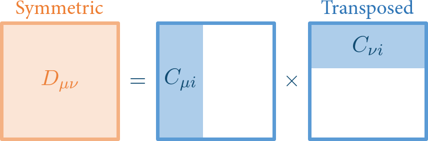
Notice that not all orbital coefficient are taken into account. Only occupied molecular orbital coefficients is included.
In the figure above, matrix in the middle is the usual representation of orbital coefficients \(C_{\mu p}\), where row denotes atomic orbital subscript \(\mu\), and column denotes molecular orbital subscript \(\nu\). For water molecule, there are 10 electrons, so number of occupied orbitals is 10/2 = 5. So only the first 5 columns (area painted in blue) is considered as \(C_{\mu i}\).
We don’t have a function determining number of occupied orbitals so far. So the reader is encouraged to implement a simple function to do this job.
Implementation
Reader should fill all NotImplementedError in the following code:
def obtain_nocc(mole: Molecule):
    # Attribute Modification: `nocc` occupied orbital
    raise NotImplementedError("About 1~5 lines of code")

Molecule.obtain_nocc = obtain_nocc
def make_rdm1(mole: Molecule, coeff: np.ndarray) -> np.ndarray:
    # Input: molecular orbital coefficient
    # Output: density for the given orbital coefficient
    raise NotImplementedError("About 1~5 lines of code")

Molecule.make_rdm1 = make_rdm1
Solution
We may use the Fock matrix coeff generated in Step 6 to test whether our function works correctly.
sol_mole.obtain_nocc()
coeff = sol_mole.get_coeff_from_fock_diag(sol_mole.get_fock(dm_random))
sol_mole.make_rdm1(coeff)
array([[ 2.1025753, -0.5617635, -0.1258392, -0.0152828,  0.2076956,  0.2044125,  0.0194752],
       [-0.5617635,  2.4763685,  0.8043683,  0.489414 ,  0.0651585, -1.229321 , -0.1506671],
       [-0.1258392,  0.8043683,  0.955106 , -0.0543459,  0.1394193, -0.3645514, -0.7655245],
       [-0.0152828,  0.489414 , -0.0543459,  2.1082959, -0.444352 , -0.5733756, -0.6135682],
       [ 0.2076956,  0.0651585,  0.1394193, -0.444352 ,  0.1910204, -0.2730566,  0.0491367],
       [ 0.2044125, -1.229321 , -0.3645514, -0.5733756, -0.2730566,  2.5931491,  0.2283302],
       [ 0.0194752, -0.1506671, -0.7655245, -0.6135682,  0.0491367,  0.2283302,  1.0875576]])
Step 8: Update Density Matrix
Review procedure from Step 5 to Step 7:
Step 5: \(D_{\mu \nu} \rightarrow F_{\mu \nu}\)
Step 6: \(F_{\mu \nu} \rightarrow C_{\mu p}\)
Step 7: \(C_{\mu p} \rightarrow D_{\mu \nu}\)
Run these processes in series, and the density updated. If we just simply loop these three steps infinitely, then we except the density converged to stable, i.e. self-consistent.
Write a function that inputs a guess density matrix, output an updated density matrix.
Implementation
Reader should fill all NotImplementedError in the following code:
def get_updated_dm(mole: Molecule, dm: np.ndarray) -> np.ndarray:
    # Input: Guess density matrix
    # Output: Updated density matrix
    raise NotImplementedError("About 1~5 lines of code")

Molecule.get_updated_dm = get_updated_dm
Solution
We use the random-generated density matrix dm_random in Step 5 to test whether our function works correctly.
sol_mole.get_updated_dm(dm_random)
array([[ 2.1025753, -0.5617635, -0.1258392, -0.0152828,  0.2076956,  0.2044125,  0.0194752],
       [-0.5617635,  2.4763685,  0.8043683,  0.489414 ,  0.0651585, -1.229321 , -0.1506671],
       [-0.1258392,  0.8043683,  0.955106 , -0.0543459,  0.1394193, -0.3645514, -0.7655245],
       [-0.0152828,  0.489414 , -0.0543459,  2.1082959, -0.444352 , -0.5733756, -0.6135682],
       [ 0.2076956,  0.0651585,  0.1394193, -0.444352 ,  0.1910204, -0.2730566,  0.0491367],
       [ 0.2044125, -1.229321 , -0.3645514, -0.5733756, -0.2730566,  2.5931491,  0.2283302],
       [ 0.0194752, -0.1506671, -0.7655245, -0.6135682,  0.0491367,  0.2283302,  1.0875576]])
Step 9: Compute the Total Energy
Compute the total energy as (Szabo and Ostlund, eq 3.184 - 3.185)
where \(F_{\mu \nu}\) is obtained from the the same density matrix \(D_{\mu \nu}\) in the fomular above. Indeed, \(E_\mathrm{tot}\) could be regarded as a function of density matrix \(D_{\mu \nu}\). \(E_\mathrm{nuc}\) has been already obtained in Step 1.
Implementation
Reader should fill all NotImplementedError in the following code:
def eng_total(mole: Molecule, dm: np.ndarray) -> float:
    # Input: Any density matrix (although one should impose tr(D@S)=nelec to satisfy variational principle)
    # Output: SCF energy (electronic contribution + nuclear repulsion contribution)
    raise NotImplementedError("About 1~5 lines of code")

Molecule.eng_total = eng_total
Solution
We use the random-generated density matrix dm_random in Step 5 to test whether our function works correctly.
sol_mole.eng_total(dm_random)
-126.934270832249
Warning
You may find the converged energy is about -75 Hartree (a.u.). Maybe to you, it is very suspicious that some density could yield much lower energy (-127) than the variational minimum (-75). This is because the density dm_random does not satisfy boundary condition \(\mathrm{tr} (\mathbf{DS}) = n_\mathrm{elec}\).
Step 10: SCF Loop and Convergence
Given initial (empty) density \(D_{\mu \nu}^0 = 0\) and initial energy value \(E_\mathrm{tot}^0 = 0\). Use the function described in Step 9 to update density matrix until convergence.
What defines convergence is energy and density criterion:
where superscript \(t\) means self-consistent field loop iteration. \(\mathrm{rms}_\mathbf{D}\) is actually Frobenius norm of the difference in consecutive density matrix.
In our implementation, we set criterion
and maximum iteration number set to 64.
Implementation
Reader should fill all NotImplementedError in the following code:
def scf_process(mole: Molecule, dm_guess: np.ndarray=None) -> Tuple[float, np.ndarray]:
    # Input: Density matrix guess
    # Output: Converged SCF total energy and density matrix
    eng, dm = 0., np.zeros((mole.nao, mole.nao)) if dm_guess is None else np.copy(dm_guess)
    eng_next, dm_next = NotImplemented, NotImplemented
    max_iter, thresh_eng, thresh_dm = 64, 1e-10, 1e-8
    print("{:>5} {:>20} {:>20} {:>20}".format("Epoch", "Total Energy", "Energy Deviation", "Density Deviation"))
    for epoch in range(max_iter):
        raise NotImplemented("Calculate total energy and update density. About 2 lines of code")
        print("{:5d} {:20.12f} {:20.12f} {:20.12f}".format(epoch, eng_next, eng_next - eng, np.linalg.norm(dm_next - dm)))
        raise NotImplemented("Test convergence criterion and judge if we should break. About 2 lines of code")
        eng, dm = eng_next, dm_next
    return eng, dm
Solution
dm_guess = np.zeros((sol_mole.nao, sol_mole.nao))
eng_converged, dm_converged = sol_mole.scf_process(dm_guess)
eng_converged, dm_converged
Epoch         Total Energy     Energy Deviation    Density Deviation
    0       8.002367061811       8.002367061811       5.100522155128
    1     -73.285796421100     -81.288163482911       3.653346168960
    2     -74.828125379745      -1.542328958644       0.959140729724
    3     -74.935487998012      -0.107362618267       0.173663377814
    4     -74.941477742494      -0.005989744483       0.062052272719
    5     -74.941971996116      -0.000494253622       0.021598566359
    6     -74.942056061414      -0.000084065298       0.010509653663
    7     -74.942074419139      -0.000018357725       0.004877159285
    8     -74.942078647640      -0.000004228501       0.002354559061
    9     -74.942079630140      -0.000000982500       0.001129086359
   10     -74.942079858804      -0.000000228664       0.000544409983
   11     -74.942079912038      -0.000000053234       0.000262360618
   12     -74.942079924431      -0.000000012394       0.000126551333
   13     -74.942079927317      -0.000000002885       0.000061045094
   14     -74.942079927988      -0.000000000672       0.000029451693
   15     -74.942079928145      -0.000000000156       0.000014209673
   16     -74.942079928181      -0.000000000036       0.000006856052
   17     -74.942079928190      -0.000000000008       0.000003308028
   18     -74.942079928192      -0.000000000002       0.000001596130
   19     -74.942079928192      -0.000000000000       0.000000770138
   20     -74.942079928192      -0.000000000000       0.000000371595
   21     -74.942079928192      -0.000000000000       0.000000179297
   22     -74.942079928192       0.000000000000       0.000000086512
   23     -74.942079928192      -0.000000000000       0.000000041742
   24     -74.942079928192       0.000000000000       0.000000020141
   25     -74.942079928192      -0.000000000000       0.000000009718
(-74.94207992819236,
 array([[ 2.1097473, -0.4655955, -0.       ,  0.1052458,  0.       , -0.0163012, -0.0163012],
        [-0.4655955,  2.0302217, -0.       , -0.5646001, -0.       , -0.0610789, -0.0610789],
        [-0.       , -0.       ,  0.7375898,  0.       , -0.       ,  0.5501973, -0.5501973],
        [ 0.1052458, -0.5646001,  0.       ,  1.1320837,  0.       ,  0.51723  ,  0.51723  ],
        [ 0.       , -0.       , -0.       ,  0.       ,  2.       ,  0.       , -0.       ],
        [-0.0163012, -0.0610789,  0.5501973,  0.51723  ,  0.       ,  0.6690534, -0.1517744],
        [-0.0163012, -0.0610789, -0.5501973,  0.51723  , -0.       , -0.1517744,  0.6690534]]))
Addition 1: Dipole Moment
As discussed in detail in Ch. 3 of the text by Szabo and Ostlund, the calculation of one-electron properties requires density matrix and the relevant property integrals. The electronic contribution to the electric-dipole moment may be computed using (Szabo and Ostlund, eq 3.190 - 3.192)
Hint 1: Access to integrals
Integral \((\mu | \boldsymbol{r} | \nu)\) is stored in \(\boldsymbol{r}\)’s three components \((x, y, z)\). \(x\) component is stored in file input/h2o/STO-3G/mux.dat. For PySCF users, simply feed "int1e_r" to pyscf.gto.Mole.intor and integral \((\mu | \boldsymbol{r} | \nu)\) is returned in dimension \((3, n_\mathrm{AO}, n_\mathrm{AO})\).
Implementation
Reader should fill all NotImplementedError in the following code:
def integral_dipole(mole: Molecule) -> np.ndarray:
    # Output: Dipole related integral (mu|r|nu) in dimension (3, nao, nao)
    raise NotImplementedError("About 1~5 lines of code")

Molecule.integral_dipole = integral_dipole
def get_dipole(mole: Molecule, dm: np.array) -> np.ndarray:
    # Input: SCF converged density matrix
    # Output: Molecule dipole in A.U.
    raise NotImplementedError("About 1~5 lines of code")

Molecule.get_dipole = get_dipole
Solution
sol_mole.integral_dipole()
array([[[ 0.       ,  0.       ,  0.0507919,  0.       ,  0.       ,  0.0022297, -0.0022297],
        [ 0.       ,  0.       ,  0.6411728,  0.       ,  0.       ,  0.2627425, -0.2627425],
        [ 0.0507919,  0.6411728,  0.       ,  0.       ,  0.       ,  0.4376306,  0.4376306],
        [ 0.       ,  0.       ,  0.       ,  0.       ,  0.       ,  0.1473994, -0.1473994],
        [ 0.       ,  0.       ,  0.       ,  0.       ,  0.       ,  0.       ,  0.       ],
        [ 0.0022297,  0.2627425,  0.4376306,  0.1473994,  0.       ,  1.6380368, -0.       ],
        [-0.0022297, -0.2627425,  0.4376306, -0.1473994,  0.       ,  0.       , -1.6380368]],

       [[-0.1432258, -0.0339021,  0.       ,  0.0507919,  0.       , -0.0037587, -0.0037587],
        [-0.0339021, -0.1432258,  0.       ,  0.6411728,  0.       ,  0.1499719,  0.1499719],
        [ 0.       ,  0.       , -0.1432258,  0.       ,  0.       ,  0.1089522, -0.1089522],
        [ 0.0507919,  0.6411728,  0.       , -0.1432258,  0.       ,  0.3340907,  0.3340907],
        [ 0.       ,  0.       ,  0.       ,  0.       , -0.1432258,  0.       ,  0.       ],
        [-0.0037587,  0.1499719,  0.1089522,  0.3340907,  0.       ,  1.1365488,  0.206579 ],
        [-0.0037587,  0.1499719, -0.1089522,  0.3340907,  0.       ,  0.206579 ,  1.1365488]],

       [[ 0.       ,  0.       ,  0.       ,  0.       ,  0.0507919,  0.       ,  0.       ],
        [ 0.       ,  0.       ,  0.       ,  0.       ,  0.6411728,  0.       ,  0.       ],
        [ 0.       ,  0.       ,  0.       ,  0.       ,  0.       ,  0.       ,  0.       ],
        [ 0.       ,  0.       ,  0.       ,  0.       ,  0.       ,  0.       ,  0.       ],
        [ 0.0507919,  0.6411728,  0.       ,  0.       ,  0.       ,  0.248968 ,  0.248968 ],
        [ 0.       ,  0.       ,  0.       ,  0.       ,  0.248968 ,  0.       ,  0.       ],
        [ 0.       ,  0.       ,  0.       ,  0.       ,  0.248968 ,  0.       ,  0.       ]]])
sol_mole.get_dipole(dm_converged)
array([0. , 0.6035213, 0. ])
Addition 2: Mulliken Population Analysis
A Mulliken population analysis (also described in Szabo and Ostlund, Ch. 3) requires the overlap integrals and the electron density, in addition to information about the number of basis functions centered on each atom. The charge on atom A may be computed as (Szabo and Ostlund, eq 3.196)
where the summation is limited to only those basis functions centered on atom \(A\).
PySCF Approach
Due to limited file input, this task could only be accomplished by the help from PySCF. Function pyscf.gto.Mole.aoslice_by_atom could help group atomic orbitals by its atom center.
Implementation
This task is a little difficult, due to \(\mu \in A\) is hard to figure out by program. So this task is not required to be accomplished by one’s own. However, hard-coding is possible for a specified system, for example water/STO-3G.
Reader may try to fill NotImplementedError in the following code:
def population_analysis(mole: Molecule, dm: np.array) -> np.ndarray:
    # Input: SCF converged density matrix
    # Output: Mulliken population analysis, charges on every atom
    raise NotImplementedError("About 5~10 lines of code")

Molecule.population_analysis = population_analysis
Solution
sol_mole.population_analysis(dm_converged)
array([-0.2531461, 0.126573 , 0.126573 ])
Test Cases
Water/STO-3G (Directory)
sol_mole = SolMol()
sol_mole.construct_from_dat_file("input/h2o/STO-3G/geom.dat")
sol_mole.obtain_mol_instance(basis="STO-3G")
sol_mole.obtain_nocc()
sol_mole.path_dict = {
    "enuc": "input/h2o/STO-3G/enuc.dat",
    "s":    "input/h2o/STO-3G/s.dat",
    "t":    "input/h2o/STO-3G/t.dat",
    "v":    "input/h2o/STO-3G/v.dat",
    "eri":  "input/h2o/STO-3G/eri.dat",
    "mux":  "input/h2o/STO-3G/mux.dat",
    "muy":  "input/h2o/STO-3G/muy.dat",
    "muz":  "input/h2o/STO-3G/muz.dat",
}
sol_mole.obtain_nao(file_path=sol_mole.path_dict["s"])
sol_mole.print_solution_03()
=== SCF Process ===
Epoch         Total Energy     Energy Deviation    Density Deviation
    0       8.002367061811       8.002367061811       5.100522155128
    1     -73.285796421100     -81.288163482911       3.653346168960
    2     -74.828125379745      -1.542328958644       0.959140729724
    3     -74.935487998012      -0.107362618267       0.173663377814
    4     -74.941477742494      -0.005989744483       0.062052272719
    5     -74.941971996116      -0.000494253622       0.021598566359
    6     -74.942056061414      -0.000084065298       0.010509653663
    7     -74.942074419139      -0.000018357725       0.004877159285
    8     -74.942078647640      -0.000004228501       0.002354559061
    9     -74.942079630140      -0.000000982500       0.001129086359
   10     -74.942079858804      -0.000000228664       0.000544409983
   11     -74.942079912038      -0.000000053234       0.000262360618
   12     -74.942079924431      -0.000000012394       0.000126551333
   13     -74.942079927317      -0.000000002885       0.000061045094
   14     -74.942079927988      -0.000000000672       0.000029451693
   15     -74.942079928145      -0.000000000156       0.000014209673
   16     -74.942079928181      -0.000000000036       0.000006856052
   17     -74.942079928190      -0.000000000008       0.000003308028
   18     -74.942079928192      -0.000000000002       0.000001596130
   19     -74.942079928192      -0.000000000000       0.000000770138
   20     -74.942079928192      -0.000000000000       0.000000371595
   21     -74.942079928192      -0.000000000000       0.000000179297
   22     -74.942079928192       0.000000000000       0.000000086512
   23     -74.942079928192      -0.000000000000       0.000000041742
   24     -74.942079928192       0.000000000000       0.000000020141
   25     -74.942079928192      -0.000000000000       0.000000009718
=== Dipole (in A.U.) ===
[0.        0.6035213 0.       ]
=== Mulliken Population Analysis ===
[-0.2531461  0.126573   0.126573 ]
Water/DZ (Directory)
sol_mole = SolMol()
sol_mole.construct_from_dat_file("input/h2o/DZ/geom.dat")
sol_mole.obtain_mol_instance(basis="DZ")
sol_mole.obtain_nocc()
sol_mole.path_dict = {
    "enuc": "input/h2o/DZ/enuc.dat",
    "s":    "input/h2o/DZ/s.dat",
    "t":    "input/h2o/DZ/t.dat",
    "v":    "input/h2o/DZ/v.dat",
    "eri":  "input/h2o/DZ/eri.dat",
    "mux":  "input/h2o/DZ/mux.dat",
    "muy":  "input/h2o/DZ/muy.dat",
    "muz":  "input/h2o/DZ/muz.dat",
}
sol_mole.obtain_nao(file_path=sol_mole.path_dict["s"])
# sol_mole.print_solution_03()
sol_mole.mol._basis
{'H': [[0, [19.2406, 0.032828], [2.8992, 0.231208], [0.6534, 0.817238]],
  [0, [0.1776, 1.0]]],
 'O': [[0,
   [7816.54, 0.002031],
   [1175.82, 0.015436],
   [273.188, 0.073771],
   [81.1696, 0.247606],
   [27.1836, 0.611832],
   [3.4136, 0.241205]],
  [0, [9.5322, 1.0]],
  [0, [0.9398, 1.0]],
  [0, [0.2846, 1.0]],
  [1,
   [35.1832, 0.01958],
   [7.904, 0.124189],
   [2.3051, 0.394727],
   [0.7171, 0.627375]],
  [1, [0.2137, 1.0]]]}
Water/DZP (Directory) For this molecule, read-input approach is prefered. For explanation, see comment in code.
sol_mole = SolMol()
sol_mole.construct_from_dat_file("input/h2o/DZP/geom.dat")
sol_mole.obtain_mol_instance(basis="DZP_Dunning")
# The following 3 lines of code is only used to reproduce the exact integral values
# That is using cartesian orbital (d shell), and one s orbital of H atom become more diffuse
# Guess the original Crawford project is psi3-era, since this basis is psi3-dzp.gbs in psi4
# The reader could just take these 3 lines without any consideration now
sol_mole.mol._basis["H"][2][1][0] = 0.75
sol_mole.mol.cart = True
sol_mole.mol.build()
sol_mole.obtain_nocc()
sol_mole.path_dict = {
    "enuc": "input/h2o/DZP/enuc.dat",
    "s":    "input/h2o/DZP/s.dat",
    "t":    "input/h2o/DZP/t.dat",
    "v":    "input/h2o/DZP/v.dat",
    "eri":  "input/h2o/DZP/eri.dat",
    "mux":  "input/h2o/DZP/mux.dat",
    "muy":  "input/h2o/DZP/muy.dat",
    "muz":  "input/h2o/DZP/muz.dat",
}
sol_mole.obtain_nao(file_path=sol_mole.path_dict["s"])
sol_mole.print_solution_03()
=== SCF Process ===
Epoch         Total Energy     Energy Deviation    Density Deviation
    0       8.002367061811       8.002367061811       6.257265233492
    1     -69.170053861694     -77.172420923505      17.801143659997
    2     -71.415303617369      -2.245249755675      17.110557111597
    3     -73.721678035341      -2.306374417971       5.307965471502
    4     -74.381838191510      -0.660160156170       4.571348737722
    5     -75.161436131461      -0.779597939951       2.439102528531
    6     -75.510928746774      -0.349492615314       1.930041242703
    7     -75.762675155351      -0.251746408577       1.232205113151
    8     -75.879680085321      -0.117004929970       0.916128789513
    9     -75.946361719726      -0.066681634405       0.613780446754
   10     -75.977561890457      -0.031200170731       0.442401057269
   11     -75.993744120619      -0.016182230162       0.301602891297
   12     -76.001410814858      -0.007666694239       0.213952051504
   13     -76.005239911770      -0.003829096912       0.147280173556
   14     -76.007073420274      -0.001833508504       0.103604143871
   15     -76.007975034687      -0.000901614413       0.071717537053
   16     -76.008409647227      -0.000434612540       0.050226193234
   17     -76.008621929669      -0.000212282442       0.034875554059
   18     -76.008724632743      -0.000102703074       0.024367318109
   19     -76.008774643915      -0.000050011172       0.016948253356
   20     -76.008798885129      -0.000024241215       0.011826975181
   21     -76.008810672478      -0.000011787348       0.008233394702
   22     -76.008816391373      -0.000005718895       0.005741738436
   23     -76.008819170302      -0.000002778929       0.003999031169
   24     -76.008820519187      -0.000001348884       0.002787846838
   25     -76.008821174422      -0.000000655235       0.001942180465
   26     -76.008821492544      -0.000000318122       0.001353705229
   27     -76.008821647050      -0.000000154506       0.000943197655
   28     -76.008821722072      -0.000000075022       0.000657347543
   29     -76.008821758507      -0.000000036434       0.000458041038
   30     -76.008821776199      -0.000000017692       0.000319208407
   31     -76.008821784790      -0.000000008592       0.000222433401
   32     -76.008821788962      -0.000000004172       0.000155009394
   33     -76.008821790989      -0.000000002026       0.000108017071
   34     -76.008821791972      -0.000000000984       0.000075273839
   35     -76.008821792450      -0.000000000478       0.000052454539
   36     -76.008821792682      -0.000000000232       0.000036553701
   37     -76.008821792795      -0.000000000113       0.000025472575
   38     -76.008821792850      -0.000000000055       0.000017750857
   39     -76.008821792876      -0.000000000027       0.000012369785
   40     -76.008821792889      -0.000000000013       0.000008620007
   41     -76.008821792895      -0.000000000006       0.000006006911
   42     -76.008821792898      -0.000000000003       0.000004185970
   43     -76.008821792900      -0.000000000001       0.000002917024
   44     -76.008821792901      -0.000000000001       0.000002032754
   45     -76.008821792901      -0.000000000000       0.000001416540
   46     -76.008821792901      -0.000000000000       0.000000987128
   47     -76.008821792901       0.000000000000       0.000000687888
   48     -76.008821792901      -0.000000000000       0.000000479360
   49     -76.008821792901       0.000000000000       0.000000334046
   50     -76.008821792901      -0.000000000000       0.000000232783
   51     -76.008821792901      -0.000000000000       0.000000162217
   52     -76.008821792901       0.000000000000       0.000000113042
   53     -76.008821792901       0.000000000000       0.000000078774
   54     -76.008821792901      -0.000000000000       0.000000054894
   55     -76.008821792901       0.000000000000       0.000000038254
   56     -76.008821792901      -0.000000000000       0.000000026657
   57     -76.008821792901      -0.000000000000       0.000000018576
   58     -76.008821792901       0.000000000000       0.000000012945
   59     -76.008821792901      -0.000000000000       0.000000009021
=== Dipole (in A.U.) ===
[-0.         0.9026624 -0.       ]
=== Mulliken Population Analysis ===
[-0.6109947  0.3054973  0.3054973]
Methane/STO-3G (Directory)
sol_mole = SolMol()
sol_mole.construct_from_dat_file("input/ch4/STO-3G/geom.dat")
sol_mole.obtain_mol_instance(basis="STO-3G")
sol_mole.obtain_nocc()
sol_mole.path_dict = {
    "enuc": "input/ch4/STO-3G/enuc.dat",
    "s":    "input/ch4/STO-3G/s.dat",
    "t":    "input/ch4/STO-3G/t.dat",
    "v":    "input/ch4/STO-3G/v.dat",
    "eri":  "input/ch4/STO-3G/eri.dat",
    "mux":  "input/ch4/STO-3G/mux.dat",
    "muy":  "input/ch4/STO-3G/muy.dat",
    "muz":  "input/ch4/STO-3G/muz.dat",
}
sol_mole.obtain_nao(file_path=sol_mole.path_dict["s"])
sol_mole.print_solution_03()
=== SCF Process ===
Epoch         Total Energy     Energy Deviation    Density Deviation
    0      13.497304462033      13.497304462033       6.515740378275
    1     -36.083448573242     -49.580753035275       6.436541620173
    2     -39.564513419144      -3.481064845902       1.104568450885
    3     -39.721836323727      -0.157322904583       0.195127470881
    4     -39.726692997946      -0.004856674219       0.034000759430
    5     -39.726845353413      -0.000152355467       0.006127229495
    6     -39.726850157495      -0.000004804082       0.001066349141
    7     -39.726850311142      -0.000000153647       0.000197843234
    8     -39.726850316180      -0.000000005038       0.000034671446
    9     -39.726850316352      -0.000000000173       0.000006876790
   10     -39.726850316359      -0.000000000006       0.000001267090
   11     -39.726850316359      -0.000000000000       0.000000281235
   12     -39.726850316359       0.000000000000       0.000000057836
   13     -39.726850316359       0.000000000000       0.000000014097
   14     -39.726850316359      -0.000000000000       0.000000003204
=== Dipole (in A.U.) ===
[-0.  0.  0.]
=== Mulliken Population Analysis ===
[-0.2604309  0.0651077  0.0651077  0.0651077  0.0651077]
References
Szabo, A.; Ostlund, N. S. Modern Quantum Chemistry: Introduction to Advanced Electronic Structure Theory Dover Publication Inc., 1996.
ISBN-13: 978-0486691862